The fundamental components of the toolkit are written in C++. Users can build an entire system in C++. In addition to the C++ program interface, the BTK and Millennium ASR provide the Python interface produced by SWIG. Programming in Python is much easier although it takes more computational time. The toolkit was developed on Linux platforms. We confirmed that they worked on Suse, Debian and Ubuntu Linux as well as Mac OS.

Installation

Prerequisite Software

To build the BTK, we need to install the following software packages:

· Python - scripting language interpreter

· Numpy - Matlab like extension to python

· GSL - GNU Scientific Library

· SWIG - simplified wrapper and interface generator

· Autoconf - automatic project configuration

· pkg-config - automatic project configuration

· libsndfile – C library for the sound file IO

The following dependencies are optional. If they are installed on your machine, 'autoconf' will find them, then compile and link against them.

· FFTW3, FFTW-float, FFTW-thread - optimized FFT computation

· ATLAS – Automatically tuned algebra software with an efficient BLAS implementation.

Those packages are available with major Linux releases. An easy way of installing a software package is to use ‘apt-get’. To check whether the package is available or not, you can execute ‘apt-cache search’. For example, when you type ‘apt-cache search gsl’ on the command line, a Linux system will typically list the following GSL packages:

libgsl0-dbg - GNU Scientific Library (GSL) -- debug symbols package

libgsl0-dev - GNU Scientific Library (GSL) -- development package

libgsl0ldbl - GNU Scientific Library (GSL) -- library package

Then, you execute ‘apt-get install libgsl0-dev’ to install the GSL development package.

When the software packages were installed in your local directory not the system path, you have to add your installation path to the environment variable in ‘.bashrc’ as

export PKG_CONFIG_PATH=${your installation directory}/pkgconfig

If you use the ‘csh’ shell system, add the line to ‘.cshrc’, as

setenv PKG_CONFIG_PATH ${your installation directory}/pkgconfig

Getting BTK

In order to download the latest version of the source code from the SVN for the first time, type

svn checkout svn://svn.code.sf.net/p/distantspeechrecognition/code/ ./

cd trunk/btk

If you have an existing working directory that you would like to update, type

svn update .

You can also download the tar archive from our sourceforge site.

Building BTK

If you would like to install the optimized BTK in some local directory, type for example

cd ~/src/btk

./autogen.sh --force

./configure --prefix=${HOME} CFLAGS='-O4' CXXFLAGS='-O4' CPPFLAGS='-O4' SWIGFLAGS='-O'

where ${HOME} is your home directory.

If you want to use the ATLAS blas library, configure with

./configure --with-atlas=<path-to-atlas>

To build and install the BTK, type

make

make install

Setting Environment Variables

In order for C++ and Python to be able to dynamically link the BTK module, the BTK libraries have to be on the path specified with two environment variables, LD_LIBRARY_PATH and PYTHONPATH. If you have installed the BTK locally as described above and you are using 'bash', add the lines

export LD_LIBRARY_PATH =${HOME}/lib:/usr/local/lib:/usr/lib

export PYTHONPATH=${HOME}/lib/python2.6/site-packages:/usr/local/lib/python2.6/site-packages:/usr/lib/python2.6/site-packages

to your .bashrc file. If you are using 'csh', add the lines

setenv LD_LIBRARY_PATH =${HOME}/lib:/usr/local/lib:/usr/lib

setenv PYTHONPATH ${HOME}/lib/python2.6/site-packages:/usr/local/lib/python2.6/site-packages:/usr/lib/python2.6/site-packages

to your '.cshrc' file.

To test that everything has been built and installed correctly, start the Python interpreter and import the BTKJ module as

>>>import btk.modulated

If you get another Python prompt, everything has worked correctly.

User Manual

Introduction

Example scripts can be downloaded from the sourceforge.

Subband Processing

Here we describe a sample script for reconstructing a speech signal with oversampled uniform DFT filter banks.

Figure 1 shows a schematic of a modulated filter bank with M subbands and a decimation factor of D. Note that the decimation factor D corresponds to the frame shift in the overlap add/save method.

First, you need to design a filter prototype for the filter bank system. The BTK provides the scripts for several filter bank design algorithms such as [1] [2]. You can find them in “btk/tools/filterbank”. It was shown in [2] that the Nyquist(M) filter bank led to the highest speech recognition accuracy. The Nyquist(M) filter prototype can be generated with a script saved as “btk/tools/filterbank/DesignNyquistFilterBank.m”. The resultant file produced with the Matlab script needs to be converted to a binary file for Python modules. That can be done with “btk/tools/filterbank/convertPythonBin.py”. The BTK also provides examples of the filter prototype; you can find them in “btk/examples/prototypes/Nyquist”.

Figure 1 also shows the relationship between the Python object and process in adaptive subband processing. To implement the subband processing system, first import the necessary BTK modules in Python as:

>>import pickle

>>from btk.feature import *

>>from btk.modulated import *

In order to handle the input audio signal from a file “inputfilename.wav”, you instantiate a SampleFeaturePtr() object as

>>sampleFeature = SampleFeaturePtr( blockLen=128, shiftLen=128, padZeros=False )

>>sampleFeature.read( fn=’inputfilename.wav’)

You will process a block of 128 audio samples at a frame and shift the block to the next 128 samples. Then, you might want to load the coefficients of the analysis and synthesis filter prototypes from the binary files as

>>fp = open('btk/examples/prototypes/Nyquist/h-M=256-m=4-r=1.txt', 'r')

>>h_fb = pickle.load(fp)

>>fp.close()

>>fp = open('/btk/examples/prototypes/Nyquist/g-M=256-m=4-r=1.txt', 'r')

>>g_fb = pickle.load(fp)

>>fp.close()

Here, the number of subbands M is 256, the filter length factor is 2, and the exponential decimation factor is 1. Next, you need to build the instances of the analysis and synthesis filter bank systems as

>>analysisFB = OverSampledDFTAnalysisBankPtr(sampleFeature, prototype=h_fb, M=256, m=4, r=1, delayCompensationType=2 )

>>synthesisFB = OverSampledDFTSynthesisBankPtr(analysisFB, prototype=g_fb, M=256, m=4, r=1, delayCompensationType=2, gainFactor=128 )

Note that the filter bank objects need to be configured with the consistent filter prototype parameters. The OverSampledDFTAnalysisBankPtr() object corresponds to the block of analysis filtering in Figure 1. The OverSampledDFTSynthesisBankPtr() object is associated with the synthesis filtering block. The dependency between two objects is usually created by feeding an instance to the other. In the above example, the OverSampledDFTAnalysisBankPtr() takes the sampleFeature instance as an input. The analysisFB instance is given to the object for the OverSampledDFTSynthesisBankPtr().

The output of the analysis filter bank is obtained through OverSampledDFTAnalysisBankPtr().next(). Those outputs will be, for example, processed with a beamforming technique which is described in the next section. To reconstruct the signal in the time domain, repeat calling the next() iterator of the synthesis filter bank:

>>import numpy

>>soundFileWriter = WriteSoundFilePtr( fn='out.wav', sampleRate=16000, nChan=1 )

>>for b in synthesisFB:

>> soundFileWriter.writeInt( numpy.array( b, numpy.float ) )

This code will save the output data as a file. Due to the dependency generated above, the execution of the iterator of OverSampledDFTSynthesisBankPtr() calls every iterator implemented in all the dependent objects, SampleFeaturePtr() and OverSampledDFTAnalysisBankPtr(). The iterator should be implemented as the next() method in the Python or C++ source codes

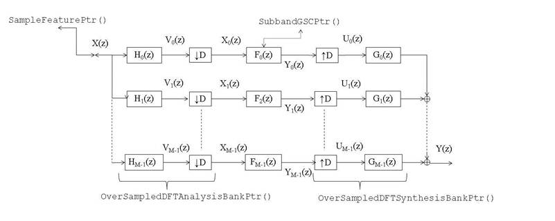
Figure 1: Block chart of a modulated subband analysis and synthesis filter bank system

Speaker Tracking

One of the attractive microphone array applications is perhaps a sound source localizer. It is the first step to enhance distant speech. The BTK implements a speaker tracking method with Kalman filtering [3]. In the speaker tracking method, time delays estimated through the phase transformation are associated with the state vector. The speaker’s position is then mapped to the observation vector. The method can interpolate the trajectory of the speaker’s position well even with 16000 kHz audio.

Tracking with Linear Array

A sample script that processes the Kinect 16 kHz data can be downloaded from http://distantspeechrecognition.sourceforge.net/samples/SingleSpeakerTrackingSample.py. An audio file recorded with the Kinect is also available from http://distantspeechrecognition.sourceforge.net/samples/ KINECT_M1001_U1050_2M.wav.

After you put the “SingleSpeakerTrackingSample.py” and “KINECT_M1001_U1050_2M.wav” in the same directory, you execute the Python script as:

>>python SingleSpeakerTrackingSample.py KINECT_M1001_U1050_2M.wav ./result/

It will show an estimate of direction of arrival (DOA) at each frame.

Delay-and-sum Beamforming

The delay-and-sum (D&S) beamforming is the most basic algorithm [4] [5]. Let us begin with the delay-and-sum beamformer. Figure 2 shows the dependency chart of the BTK objects in the case of beamforming.

Figure 2: Dependency of the BTK Objects in Beamforming

As shown in Figure 2, you first need to instantiate the sample feature and analysis filter bank objects to handle multi-channel data as

>>chanN =4 # Example of the 4-channel case

>>M=256 # No. subbands

>>m=4 # Filter length factor

>>r=1 # Exponential decimation factor

>>D= M / 2**r # Frame shift

>>allSampleFeats = []

>>allAnalysisFBs = []

>>for chX in range(chanN):

>> sampleFeature = SampleFeaturePtr( blockLen=D, shiftLen=D, padZeros=False )

>> allSampleFeats.append(sampleFeature)

>> analysisFB = OverSampledDFTAnalysisBankPtr(sampleFeature, prototype=h_fb, M=M, m=m, r=r, delayCompensationType=2 )

>> allAnalysisFBs.append(analysisFB)

Then, construct the beamformer object so as to process the multiple channels as

>>from btk.beamformer import *

>>pBeamformer = SubbandGSCPtr( fftLen=M, halfBandShift=False)

Now, as illustrated in Figure 2, we give the multiple analysis filter bank instances to the beamformer as

>>for chX in range(chanN):

>> pBeamformer.setChannel(allAnalysisFBs[chX])

Then, you load a multi-channel audio file to the SampleFeaturePtr() instance as

>>for chX in range(chanN):

>> allSampleFeats[chX].read( fn='multichannel.wav', chX=(chX + 1), chN=chanN )

Furthermore, the delay-and-sum beamformer requires the time delays of arrival of the target source. To compute the time delays, you can use the position estimates obtained with the speaker tracking script. Assuming that you obtain the direction of arrival from “direction.txt” and the uniform linear array is used, Python should read

>>import numpy

>>sampleRate = 16000

>>avgDOA = readDirectoinOfArrival('direction.txt' )

>>timedelays = numpy.zeros( chanN, numpy.float )

>>distance = 36 # mm

>>for chX in range(chanN):

>> timedelays[chX] = - distance * numpy.cos( avgDOAs ) / 343000.0

>>pBeamformer.calcGSCWeights( sampleRate, delaysL )

>>for fbinX in range(M/2+1):

>> pBeamformer.setActiveWeights_f( fbinX, numpy.zeros( 2*(chanN-1), numpy.float ) )

Here, the speed of sound is set to 343000.0 mm/s.

The last step is to reconstruct the beamformer’s ouput in the time domain. This can be done by feeding the beamformer instance to the OverSampledDFTSynthesisBankPtr() as

>>synthesisFB = OverSampledDFTSynthesisBankPtr(pBeamformer, prototype=g_fb, M=M, m=m, r=r, delayCompensationType=2, gainFactor=D )

>>soundFileWriter = WriteSoundFilePtr( fn='dsbeamformer.wav', sampleRate=sampleRate, nChan=1 )

>>for b in synthesisFB:

>> soundFileWriter.writeInt(numpy.array( b, numpy.float ) )

In the example above, we assume that the source position is static. Of course, you can change the time delay for the beamformer at each frame.

Array Post-filtering

It is well known that microphone array post-filtering can further improve noise suppression performance [6] [7] [8]. Simmer et al. showed in [6] that the minimum mean square error beamformer can be, in fact, decomposed into the Wiener filter and minimum variance distortionless response beamformer. Unfortunately, we did not observe a significant difference among post-filtering techniques in terms of speech recognition especially in the case of an array with more than 4 microphones. The BTK thus provides only popular post-filtering methods, Zelinski post-filter, McCowan [7] and Lefkimmiatis post-filters [8].

It is very easy to try post-filters with the BTK. Once you build the beamformer explained above, what you need to use the post-filter is to feed the beamformer instance to a post-filter object and plug it into the synthesis filter bank chain as

>>from btk.postfilter import *

>>alpha =0.6 # forgetting factor for the power spectrum estimation

>>postfiltertype = 2 # Use abs() for the real operator

>>output = ZelinskiPostFilterPtr( pBeamformer, fftLen, alpha, postfilterType )

>>synthesisFB = OverSampledDFTSynthesisBankPtr(output, prototype=g_fb, M=M, m=m, r=r, delayCompensationType=2, gainFactor=D )

You can reconstruct the audio signal in the same way as explained before.

Super-Directive Beamforming

In many situations such as enclosed rooms, the noise covariance (spatial correlation) matrix cannot be represented as the identity matrix. In such as case, the D&S beamformer is not the optimum solution. The super-directive (SD) beamformer often provides better noise suppression performance [9].

The SD beamformer assumes that the noise field is spherically isotropic. Intuitively, you can imagine a situation where a noise wave sound signal comes from all the directions to the array.

The BTK provides the SD beamformer. In the same way as D&S beamforming, you need to instantiate a SubbandMVDRPtr() Python object with multiple analysis filter banks and set the time delays of arrival:

>>pBeamformer = SubbandMVDRPtr( fftLen=M, halfBandShift=False )

>>for chX in range(chanN):

>> pBeamformer.setChannel(allAnalysisFBs[chX])

>>pBeamformer.calcArrayManifoldVectors( sampleRate, delaysL )

In order to compute the diffuse noise field, you tell the array geometry matrix to the beamformer instance:

>>arraygeom = numpy.array([[-113.0,0.0,2.0], [36.0,0.0,2.0], [76.0,0.0,2.0], [113.0,0.0,2.0]]) # arraygeom[chanN][3]: Columns correspond to x, y and z positions.

>>pBeamformer.setDiffuseNoiseModel(arraygeom, sampleRate, 343000.0 )

You can now compute the SD beamformer’s weight by adjusting an amount of diagonal loading as

>>pBeamformer.setAllLevelsOfDiagonalLoading( 0.01 )

>>pBeamformer.calcMVDRWeights( sampleRate, dThreshold=1.0E-8, calcInverseMatrix=True )

Minimum Variance Distortionless Response Beamforming

In many cases, the D&S and SD beamformers work well robustly. However, you might want to tune up the beamformer to a specific noise environment. It can be achieved with the minimum variance distortionless response (MVDR) beamformer. It is easy to try the MVDR beamformer with the BTK.

The first step of building the MVDR beamformer is to estimate the noise covariance matrix with an actual noise measurement. Here, we assume that we recorded background noise in a similar condition with a test environment and save it as “mc-noise.wav”. Then, the Python function to compute the noise covariance matrix can be written as:

>>def computeCovarianceMatrix( filename='mc-noise.wav', chanN=4, M=256, m=4, r=1, maxFrame=32768 ):

>> D= M / 2**r # Frame shift

>> allSampleFeats = []

>> allAnalysisFBs = []

>> for chX in range(chanN):

>> sampleFeature = SampleFeaturePtr( blockLen=D, shiftLen=D, padZeros=False )

>> sampleFeature.read( fn=filename, chX=(chX + 1), chN=chanN )

>> analysisFB = OverSampledDFTAnalysisBankPtr(sampleFeature, prototype=h_fb, M=M, m=m, r=r, delayCompensationType=2 )

>> allSampleFeats.append(sampleFeature)

>> allAnalysisFBs.append(analysisFB)

>> observations = []

>> snapShotArray = SnapShotArrayPtr( M, chanN )

>> for sX in range(maxFrame):

>> try:

>> chX = 0

>> for afb in analysisFBs:

>> snapShotArray.newSample(numpy.array(afb.next()), chX )

>> chX +=1

>> snapShotArray.update()

>> X_t = [] # X_t[fftLen][chanN]

>> for fbinX in range(M):

>> X_t.append( copy.deepcopy( snapShotArray.getSnapShot(fbinX) ) )

>> observations.append( X_t )

>> except:

>> break

>> frameN = len(observations)

>> SigmaX = numpy.zeros( (M/2+1,chanN,chanN), numpy.complex )

>> for sX in range(frameN):

>> for fbinX in range(M/2+1):

>> SigmaX[fbinX] += numpy.outer( observations[sX][fbinX], numpy.conjugate(observations[sX][fbinX]) ) / frameN

>> return SigmaX

It is a kind of cheating because we will not always get such a perfect noise segment in many applications. In practice, you have to be very careful for computing the noise covariance matrix. In the case that the noise covariance is calculated with the target signal, the resultant MVDR beamformer suppresses not only noise but also the desired signal.

After the noise covariance matrix is estimated, you need to set it to the SubbandMVDRPtr() object as:

>>pBeamformer = SubbandMVDRPtr( fftLen=M, halfBandShift=False )

>>for chX in range(chanN):

>> pBeamformer.setChannel(allAnalysisFBs[chX])

>>pBeamformer.calcArrayManifoldVectors( sampleRate, delaysL )

>>SigmaX = computeCovarianceMatrix()

>>for fbinX in range(M/2+1):

>> pBeamformer.setNoiseSpatialSpectralMatrix( fbinX, SigmaX[fbinX] )

>>pBeamformer.setAllLevelsOfDiagonalLoading( 0.01 )

>>pBeamformer.calcMVDRWeights( sampleRate, dThreshold=1.0E-8, calcInverseMatrix=True )

In the same ways as the other beamformers, you just need to plug the beamformer instance to the synthesis filter bank object and run the iterator to obtain the beamformed signal.

Minimum Mean Square Error Beamforming

For the same reason as the Wiener filter implementation, the ideal minimum mean square error (MMSE) cannot be in practice achieved with microphone arrays. One implementation way is to build the MVDR beamformer with the array post-filter as described in [6]. Another example is to compute the beamformer’s weights from the noise matrix as in [10] where the authors were actually unaware of the MMSE beamformers described in [5]. In either way, we can easily implement the MMSE beamformer with the BTK if we have an exact noise covariance matrix.

Maximum Negentropy/Kurtosis Beamforming

Another approach is to incorporate the super-Gaussianity of speech into beamforming [11]. It turned out that super-Gaussian beamforming does not suffer from signal cancellation encountered in conventional beamforming [12]. Accordingly, it does not need an accurate voice activity detector required by conventional beamforming. The BTK toolkit offers Python scripts for maximum negentropy beamforming [12].

The super-Gaussianity can be measured with the kurtosis which does not require the pre-trained speech model. The maximum kurtosis beamformer can be simply implemented with the BTK [13].

Spherical Harmonics D&S Beamforming

The spherical array is potentially capable of representing the 3D sound field more accurately [14]. Those arrays are commercially available from mh acoustics LLC and VisiSonic. The BTK also implements spherical array algorithms. John McDonough, Kenichi Kumatani and Bhiksha Raj investigated the effect of the spherical array on speech recognition through experiments with distant speech played through a loudspeaker [11, 15]. In [16], John McDonough et al. demonstrated through experiments on real distant speech that the recognition performance was improved by using the spherical array with a novel speaker tracking algorithm.

The BTK implements popular spherical harmonics beamforming methods, spherical harmonics delay-and-sum (D&S) and super-directive (SD) beamformer. To build the spherical harmonics D&S beamformer, you instantiate the SphericalDSBeamformerPtr() object and set the analysis filter banks to it as follows.

>>maxOrder = 5

>>chanN = 32

>>pBeamformer = SphericalDSBeamformerPtr( sampleRate=44100, fftLen=fftLen, halfBandShift=False, NC=1, maxOrder=maxOrder, normalizeWeight=False, ratio=0.5 )

>>pBeamformer.setEigenMikeGeometry() # mh acoustics EigenMike’s geometry

>>pBeamformer.setSigma2( 0.01 ) # WNG control

>>for chX in range(chanN):

>> pBeamformer.setChannel( allAnalysisFBs[chX] )

You then tell the beamformer instance a look direction in radians as

>>pBeamformer.setLookDirection( theta, phi )

After that, you plug the beamformer instance to the OverSampledDFTSynthesisBankPtr() and reconstruct the signal as explained above.

Spherical Harmonics SD Beamforming

In the same way as conventional SD beamforming, the spherical array can be optimized for the diffuse noise field, which was proven to work well in an indoor environment [11] [16]. The BTK also implements the spherical harmonics SD beamforming. In the same way as the spherical harmonics D&S beamformer, you construct the SphericalHWNCBeamformerPtr () object with the multiple analysis filter banks, set the look direction and feed it to the synthesis filter bank to obtain the beamformed signal.

Dereverberation

Although many people tend to forget about reverberation, it will degrade distant speech recognition performance significantly [17] [18] [19]. Dereverberation can be done through super-Gaussian beamforming [12] [13] or WPF algorithm [20]. The BTK also implements the WPF algorithm in the subband domain.

To use it in Python, import the dereverberation module as

>>import btk.dereverberation

The WPE algorithm for an single channel can be done by setting the analysis filter bank output to the SingleChannelWPEDereverberationFeaturePtr() object as follows.

>>sampleFeature = SampleFeaturePtr( blockLen=D, shiftLen=D, padZeros=False )

>>analysisFB = OverSampledDFTAnalysisBankPtr(sampleFeature, prototype=h_fb, M=M, m=m, r=r, delayCompensationType=2 )

>>output = SingleChannelWPEDereverberationFeaturePtr( analysisFB, lowerN=0, upperN=60, iterationsN=2,loadDb=-20.0, bandWidth=0.0, sampleRate=16000.0 )

>>synthesisFB = OverSampledDFTSynthesisBankPtr(output, prototype=g_fb, M=M, m=m, r=r, delayCompensationType=2, gainFactor=D )

The WPE dereverberator can be tuned by limiting the minimum and maximum delays of the reflections, upperN and lowerN. The number of prediction coefficients will be calculated with those parameters as upperN – lowerN + 1.

The multi-channel version of the WPE algorithm can be implemented with MultiChannelWPEDereverberationPtr() and MultiChannelWPEDereverberationFeaturePtr().

First, you need to build MultiChannelWPEDereverberationPtr() with the multiple analysis filer bank features. It can be done in the similar way with beamforming as

>>M=256

>>chanN=4

>>mcWPEDereverb = MultiChannelWPEDereverberationPtr( subbandsN=M, channelsN=chanN, lowerN=0, upperN=60, iterationsN=2,loadDb=-20.0, bandWidth=0.0, sampleRate=16000.0 )

>>for chX in range(chanN):

>> mcWPEDereverb.setInput( allAnalysisFBs[chX] )

After that, you need to set the instance of the MultiChannelWPEDereverberationPtr() to the MultiChannelWPEDereverberationFeaturePtr() object for each channel.

>>allSynthesisFBs = []

>>for chX in range(chanN):

>> output = MultiChannelWPEDereverberationFeaturePtr( mcWPEDereverb, channelX=chX )

>> synthesisFB = OverSampledDFTSynthesisBankPtr(output, prototype=g_fb, M=M, m=m, r=r, delayCompensationType=2, gainFactor=D )

>> allSynthesisFBs.append( synthesisFB )

The output for each channel input is reconstructed by calling the iterator of each synthesis filter bank object.

Echo Cancellation

Acoustic echo cancellation (AEC) techniques themselves are well-developed; see [21] [22] for an overview and practical algorithms. The only research theme would be how to efficiently combine AEC and multi-channel processing [23]. Generally speaking, performing AEC before beamforming provides better speech enhancement performance at the expense of computational complexity. The BTK provides the NLMS AEC [21] [22]. The BTK also implements the subband AEC with Kalman filters [24] [25] rather than the full band AEC [26].

To use the AEC, you first need to import the AEC Python module:

>>from btk.cancelVP import *

Then, you construct two analysis filter bank objects for an observed signal and a reference signal

>>obsSampFeature = SampleFeaturePtr(blockLen=D, shiftLen=D, padZeros=True)

>>obsAnalysisFB = OverSampledDFTAnalysisBankPtr(obsSampFeature, prototype=h_fb, M=M, m=m, r=r, delayCompensationType=2 )

>>refSampFeature = SampleFeaturePtr(blockLen=D, shiftLen=D, padZeros=True)

>>refAnalysisFB = OverSampledDFTAnalysisBankPtr(refSampFeature, prototype=h_fb, M=M, m=m, r=r, delayCompensationType=2 )

After that, you set those subband features to an AEC object. For example, you can use the AEC with information filtering as follows.

>>snrTh = 0.1 # if SNR > snrTh, update the filter

>>lenKF = 8 # filter length in the Kalman filter

>>diagonalLoading = 10e-4 # diagonal loading added to the information matrix

>>sigmau2 = 10e-4

>>sigmak2 = 5.0

>>beta = 0.95

>>energythreshold = 1.0E+02

>>smooth = 0.95

>>AECFeature = InformationFilterEchoCancellationFeaturePtr(refAnalysisFB, obsAnalysisFB, sampleN=lenKF, beta=beta, sigmau2=sigmau2, sigmak2=5.0, threshold=energythreshold, loading=diagonalLoading )

The sensitivity on recognition performance with respect to the information filter’s parameters was investigated in [23] [24]. As described above, you can reconstruct the echo-suppressed signal through the synthesis filter bank instantiated with the AEC object as

>>synthesisFB = OverSampledDFTSynthesisBankPtr( AECFeature, prototype=g_fb, M=M, m=m, r=r, delayCompensationType=2, gainFactor=D )

>>soundFileWriter = WriteSoundFilePtr( fn='aec.wav', sampleRate=sampleRate, nChan=1 )

>>for b in synthesisFB:

>> soundFileWriter.writeInt(numpy.array( b, numpy.float ) )

BSs

In our observation, estimating an unmixing matrix blindly has never provided better performance than beamforming approaches, at least, in terms of speech recognition on real data. Therefore, the BTK skips the BSs.

MFCC Speech Feature

The mel-frequency ceptral coefficient (MFCC) [4] is perhaps the most popular speech feature used in speech recognition. With the BTK, you can easily compute the MFCC as follows.

>>from btk.feature import *

>>fftLen = 256

>>windowLen = 256

>>windowShift = 160

>>coeffN = fftLen/2 + 1

>>melN = 30

>>sampleRate = 16000.0

>>lower = 100.0

>>upper = 6800.0

>>ncep = 13

>>sampleFeature = SampleFeaturePtr(blockLen=windowLen, shiftLen=windowShift, nm='Sample')

>>sampleStorage = StorageFeaturePtr(sampleFeature, nm='Sample Storage')

>>hammingFeature = HammingFeaturePtr(sampleStorage)

>>fftFeature = FFTFeaturePtr(hammingFeature, fftLen=fftLen)

>>powerFeature = SpectralPowerFeaturePtr(fftFeature, powN=coeffN )

>>vtlnFeature = VTLNFeaturePtr(powerFeature, coeffN=coeffN, nm='VTLN', edge=0.8, version=2 )

>>melFeature = MelFeaturePtr(vtlnFeature, powN =coeffN, filterN=melN, rate=sampleRate, low=lower, up=upper, version=2)

>>logFeature = LogFeaturePtr(melFeature)

>>cepstralFeature = CepstralFeaturePtr(logFeature, ncep=ncep, nm='Cepstral')

>>cepstralStorage = StorageFeaturePtr(cepstralFeature, nm='Cepstral Storage')

To obtain the MFCC values from an audio file, you tell the SampleFeaturePtr() the audio file path and call the iterator of the StorageFeaturePtr() as

>>sampleFeature read( fn=’inputfilename.wav’)

>>for MFCCfeature in cepstralStorage:

>> print MFCCfeature

The cepstral mean variance normalization (CMN) algorithm can be also implemented with the BTK as follows.

>>framesN = 2 * 2 + 1

>>filter = numpy.array([1, 2, 3, 2, 1], numpy.float)

>>signalPowerFeature = SignalPowerFeaturePtr(sampleStorage)

>>signalPowerStorage = StorageFeaturePtr(signalPowerFeature, nm='Signal Power Storage')

>>alogFeaure = ALogFeaturePtr(signalPowerStorage, m=1.0, a = 4.0, nm='ALog Feature')

>>alogStorage = CircularStorageFeaturePtr(alogFeaure, framesN=framesN, nm='ALog Storage')

>>filterFeature1 = FilterFeaturePtr(alogStorage, filter, nm='Filter Feature 1')

>>filterStorage = CircularStorageFeaturePtr(filterFeature1, framesN=framesN, nm='Filter Storage 1')

>>filterFeature2 = FilterFeaturePtr(filterStorage, filter, nm='Filter Feature 2')

>>filterStorage2 = StorageFeaturePtr(filterFeature2, nm='Filter Storage 2')

>>normalizeFeature= NormalizeFeaturePtr(filterStorage2, min=-0.1, max=0.5)

>>thresholdFeature= ThresholdFeaturePtr(normalizeFeature, value=1.0, thresh=0.0, mode='upper', nm='Threshold')

>>speechFeature = ThresholdFeaturePtr(thresholdFeature, value=0.0, thresh=0.0, mode='lower', nm='Speech')

>>speechStorage = StorageFeaturePtr(speechFeature, nm = 'Speech Storage')

>>meanSubFeature = MeanSubtractionFeaturePtr(cepstralStorage, speechStorage, devNormFactor=2.0, nm='MeanSub')

You can also add the delta and acceleration to it.

>>deltaFilterLen = 5

>>deltaFilter = numpy.array([-2, -1, 0, 1, 2], numpy.float)

>>circCepstralFeature = CircularStorageFeaturePtr(cepstralStorage, framesN=deltaFilterLen)

>>deltaFeature = FilterFeaturePtr(circCepstralFeature, deltaFilter, nm='Delta')

>>deltaStorage = StorageFeaturePtr(deltaFeature, nm='Delta Storage')

>>circDeltaFeature = CircularStorageFeaturePtr(deltaStorage, framesN=deltaFilterLen)

>>deltaDeltaFeature = FilterFeaturePtr(circDeltaFeature, deltaFilter, nm='DeltaDelta')

>>deltaDeltaStorage = StorageFeaturePtr(deltaDeltaFeature, nm='DD Storage')

>>mergeFeature = MergeFeaturePtr(meanSubFeature, deltaStorage, deltaDeltaStorage, nm='merge')

>>finalStorage = StorageFeaturePtr(mergeFeature, nm='Final Storage')

MVDR Speech Feature

The valleys in a spectral envelope will be often affected with noise or reverberation. Accordingly, extracting the spectral peaks is more important than modeling the valleys in speech recognition. It turned out in [27] that the warped MVDR feature extraction method is more robust against noise and reverberation because of a more accurate spectral peak model with lower resolution in the valleys. The MVDR cepstral feature can be generated with the BTK as follows.

>>from btk.feature import *

>>fftLen = 256

>>windowLen = 256

>>windowShift = 160

>>coeffN = fftLen/2 + 1

>>melN = coeffN

>>sampleRate = 16000.0

>>ncep = 20

>>mvdrOrder = 30

>>mvdrWarp = 0.4595

>>sampleFeature = SampleFeaturePtr(blockLen=windowLen, shiftLen=windowShift, nm='Sample')

>>sampleStorage = StorageFeaturePtr(sampleFeature, nm = 'Sample Storage')

>>hammingFeature = HammingFeaturePtr(sampleStorage)

>>fftFeature = FFTFeaturePtr(hammingFeature, fftLen=fftLen)

>>powerFeature = SpectralPowerFeaturePtr(fftFeature, powN=coeffN)

>>mvdrFeature = WarpMVDRFeaturePtr(hammingFeature, order=mvdrOrder, warp=mvdrWarp)

>>smoothingFeature = SpectralSmoothingPtr(mvdrFeature, powerFeature)

>>melFeature = MelFeaturePtr(smoothingFeature, powN=coeffN, filterN=melN, rate=sampleRate)

>>logFeature = LogFeaturePtr(melFeature)

>>cepstralFeature = CepstralFeaturePtr(logFeature, ncep=ncep, nm='Cepstral Feature')

>>cepstralStorage = StorageFeaturePtr(cepstralFeature, nm='Cepstral Storage')

>>warp = '1'

>>melFile = 'Filterbanks16kHz16ms129bins/VTLN.filterbank.%s' %(warp)

>>melFeature.read(melFile)

Note that the mel filter bank file has to be loaded for vocal tract length normalization. The pre-computed filter bank files can be downloaded from the DSR sourceforge. The archive also contains the Matlab script to generate the filter bank file with arbitrary parameters.

Multi-Pass Decoder

The Millennium ASR only provides the GMM-based speech recognizer [28] although many people have shifted to the DNN speech recognizer. Nonetheless, many techniques can be recycled for the DNN speech recognizer.

Developer Manual

Source Code Structure

References

[1]	K. Kumatani, J. W. McDonough, S. Schachl, D. Klakow, P. N. Garner and W. Li, "Filter bank design based on minimization of individual aliasing terms for minimum mutual information subband adaptive beamforming," in ICASSP, Las Vegas, USA, 2008.
[2]	J. M. d. Haan, N. Grbic, I. Claesson and S. E. Nordholm, "Filter bank design for subband adaptive microphone arrays," IEEE Transactions on Speech and Audio Processing, pp. 14-23, 2003.
[3]	U. Klee, T. Gehrig and J. W. McDonough, "Kalman Filters for Time Delay of Arrival-Based Source Localization," EURASIP J. Adv. Sig., 2006.
[4]	M. Woelfel and J. W. McDonough, Distant Speech Recognition, New York: Wiley, 2009.
[5]	H. L. V. Trees, Optimum Array Processing, WileyInterscience, 2002.
[6]	K. U. Simmer, J. Bitzer and C. Marro, "Post-Filtering Techniques," in Microphone Arrays, Heidelberg, Germany, Springer Verlag, 2001, pp. 39-60.
[7]	I. McCowan and H. Bourlard, "Microphone array post-filter based on noise field coherence," IEEE Transactions on Speech and Audio Processing, pp. 709-716, 2003.
[8]	S. Lefkimmiatis and P. Maragos, "A generalized estimation approach for linear and nonlinear microphone array post-filters," Speech Communication, vol. 49, pp. 7-8, 2007.
[9]	J. Bitzer and K. U. Simmer, "Superdirective Microphone Arrays," in Microphone Arrays, Heidelberg, Germany, Springer Verlag, 2001, pp. 19-38.
[10]	M. Souden, J. Benesty and S. Affes, "On optimal frequency-domain multichannel linear filtering for noise reduction," IEEE Trans. Audio, Speech, Language Process, pp. 260-276, 2010.
[11]	K. Kumatani, J. McDonough and B. Raj, "Microphone array processing for distant speech recognition: From close-talking microphones to far-field sensors," IEEE Signal Processing Magazine, pp. 127-140, 2012.
[12]	K. Kumatani, J. W. McDonough, B. Rauch, D. Klakow, P. N. Garner and W. Li, "Beamforming With a Maximum Negentropy Criterion," IEEE Transactions on Audio, Speech & Language Processing, pp. 994-1008, 2009.
[13]	K. Kumatani, J. W. McDonough, B. Rauch, P. N. Garner, W. Li and J. Dines, "Maximum kurtosis beamforming with the generalized sidelobe canceller," in INTERSPEECH, Brisbane, Australia, 2008.
[14]	J. Meyer and G. W. Elko, "Spherical Microphone Arrays for 3D Sound Recording," in Audio Signal Processing for Next-Generation Multimedia Communication Systems, 2004, pp. 67-89.
[15]	J. McDonough and K. Kumatani, "Microphone Arrays," in "Techniques for Noise Robustness in Automatic Speech Recognition", Tuomas Virtanen, Rita Singh, Bhiksha Raj (Editors), Wiley, 2012, pp. 109-157.
[16]	J. W. McDonough, K. Kumatani, T. Arakawa, K. Yamamoto and B. Raj, "Speaker tracking with spherical microphone arrays," in ICASSP, Vancouver, Canada, 2013.
[17]	I. Tashev and D. Allred, " Reverberation reduction for improved speech recognition," in Proceedings of Hands-Free Communication and Microphone Arrays, Piscataway, USA, 2005.
[18]	"REVERB Challenge," 2014. [Online]. Available: http://reverb2014.dereverberation.com/.
[19]	R. Haeb-Umbach and A. Krueger, "Reverberant Speech Recognition," in "Techniques for Noise Robustness in Automatic Speech Recognition", Tuomas Virtanen, Rita Singh, Bhiksha Raj (Editors), Wiley, 2012, pp. 251-281.
[20]	T. Yoshioka and T. Nakatani, "Generalization of multi-channel linear prediction methods for blind MIMO impulse response shortening," IEEE Trans. Audio, Speech, Language Process, p. 2707–2720, 2012.
[21]	I. Tashev, Sound Capture and Processing: Practical Approaches, Wiley, 2009.
[22]	E. Haensler and G. Schmidt, Acoustic Echo and Noise Control - A Practical Approach, Wiley Interscience, 2004.
[23]	W. Herbordt, S. Nakamura and W. Kellerman, "Joint optimization of LCMV beamforming and acoustic echo cancellation for automatic speech recognition," in ICASSP, Philadelphia, PA, USA, 2005.
[24]	J. McDonough, W. Chu, K. Kumatani, B. Raj and J. Lehman, "An Information Filter for Voice Prompt Suppression," in Asilomar, Pacific Grove, CA , 2011.
[25]	J. McDonough, K. Kumatani and B. Raj, "On the Combination of Voice Prompt Suppression with Maximum Kurtosis Beamforming," in WASPAA, New Paltz, NY, 2011.
[26]	G. Enzner and P. Vary, "Frequency-domain adaptive Kalman filter for acoustic echo control in hands-free telephones," Signal Processing, pp. 1140-1156, 2006.
[27]	M. Wölfel and J. McDonough, "Minimum variance distortionless response spectral estimation, review and refinements," IEEE Signal Processing Magazine, pp. 117-126, 2005.
[28]	J. McDonough, K. Kumatani, T. Gehrig, E. Stoimenov, U. Mayer, S. Schacht, M. Woelfel and D. Klakow, "To separate speech: A system for recognizing simultaneous speech," in Proceedings of the 4th international conference on Machine learning for multimodal interaction, Brno, Czech Republic, 2007.